Dot products and duality

Calvin: You know, I don't think math is a science, I think it's a religion.

Hobbes: A religion?

Calvin: Yeah. All these equations are like miracles. You take two numbers and when you add them, they magically become one NEW number! No one can say how it happens. You either believe it or you don't.

Traditionally, dot products are introduced very early on in a linear algebra course, typically right at the start, so it might seem strange that I've pushed them back to this point in the series.

I did this because while there is a standard way to introduce the topic, which requires nothing more than an understanding of what vectors are, a fuller understanding of the role dot products play in math can only be found under the light of linear transformations. First, let me briefly cover the standard way dot products are introduced, which I'm assuming is at least partially a review for a number of readers.

Numerical Method

Numerically, if you have two vectors of the same dimension, two lists of numbers with the same lengths, taking their dot product means pairing up all the coordinates, multiplying those pairs together, and adding the result.

For instance, two vectors of length two dotted together looks like:

\left[\begin{array}{l}1 \\ 2\end{array}\right] \cdot \left[\begin{array}{l}3 \\ 4\end{array}\right] = 1 \cdot 3+2 \cdot 4 = 11

And two vectors of length four dotted together looks like:

\left[\begin{array}{l}6 \\ 2 \\ 8 \\ 3\end{array}\right] \cdot \left[\begin{array}{l}1 \\ 8 \\ 5 \\ 3\end{array}\right] = 6 \cdot 1+2 \cdot 8+8 \cdot 5+3 \cdot 3 = 71

Geometric Interpretation

Luckily, this computation has a nice geometric interpretation. To think about the dot product of two vectors \mathbf{v} and \mathbf{w}, imagine projecting \mathbf{w} onto the line that passes through the origin and the tip of \mathbf{v}.

Multiply the length of this projection by the length of \mathbf{v}, and you have the dot product \mathbf{v} dot \mathbf{w}.

When the projection of \mathbf{w} is pointing in the opposite direction from \mathbf{v}, the dot product will actually be negative.

Notice how this means the sign of a dot product tells you how much two vectors \mathbf{v} and \mathbf{w} align.

• \mathbf{v} \cdot \mathbf{w} > 0 when they point in similar directions.
• \mathbf{v} \cdot \mathbf{w} = 0 when they are perpendicular, meaning the projection of one onto the other is the zero vector.
• \mathbf{v} \cdot \mathbf{w} < 0 when they point in opposing directions.

Which of the following statements about the image below is accurate?

Order Doesn't Matter

This geometric interpretation is very asymmetric, in that it treats the two vectors very differently. When I first learned this I was surprised that order doesn't matter, that you could instead project \mathbf{v} onto \mathbf{w} and multiply the length of the projected \mathbf{v} times the length of \mathbf{w} and get the same result.

Here's the intuition for why order doesn't matter: If \mathbf{v} and \mathbf{w} are the same length, we can leverage symmetry, since projecting \mathbf{w} onto \mathbf{v} and multiplying the length of the projection by the length of \mathbf{v} is a complete mirror image of projection \mathbf{v} onto \mathbf{w} and multiplying the length of the projection by the length of \mathbf{w}.

Now, if you scale one of them, say \mathbf{v}, by some constant like 2 so that they don't have equal length, the symmetry is broken, but let's think through how to interpret the dot product between this new vector (2 times \mathbf{v}) and \mathbf{w}.

If you think of \mathbf{w} as projected onto \mathbf{v}, the dot product (2\mathbf{v}) dot \mathbf{w} will be exactly twice the dot product \mathbf{v} dot \mathbf{w}. This is because when you scale \mathbf{v} by 2, it doesn't change the length of the projection of \mathbf{w}, but it doubles the length of the vector that you're projected onto.

On the other hand, let's say you were thinking about \mathbf{v} as getting projected onto \mathbf{w}. In that case, the length of the projection is the thing that gets scaled as we multiply \mathbf{v} by 2, while the length of the vector you're projecting onto stays constant, so the overall effect is still to just double the dot product.

So even though symmetry is broken, the effect this scaling has on the value of the dot product is the same under both interpretations.

There's also another big question other than the order: Why on earth does this numerical process of matching coordinates, multiplying pairs, and adding them together have anything to do with projection? To give a satisfactory answer, and to do full justice to the significance of the dot product, we need to unearth something deeper going on here, which often goes by the name "duality." Before getting to that, I need to spend some time talking about linear transformations from multiple dimensions to one dimension, which is the number line.

ImageVideo

These are functions that take in 2d vectors and spit out numbers, but because the transformation is linear these functions are much more restricted than your run-of-the-mill function with a 2d input and a 1d output.

Linear transformations

As with transformations in higher dimensions there are some formal properties that makes one of these functions linear. This was discussed in chapter 3, so definitely go check that out if you haven't already.

I'm going to purposefully ignore these properties here so as to not distract from our end goal, and instead focus on certain visual property that's equivalent to all the formal stuff. If you take any line of evenly spaced dots, and apply the transformation, a linear transformation will keep those dots evenly spaced once that land in the output space, which is the number line.

ImageVideo

Of course, this means that if there is some line of dots that is unevenly spaced, then the transformation is not linear.

ImageVideo

As with the cases we've seen before, one of these linear transformations is completely determined by where \hat{\imath} and \hat{\jmath} land, but this time each one simply lands on a number. So when we record where they land as the columns of a matrix, each of those columns just has a single number.

Let's walk through an example of what it means to apply one of these transformations to a vector. Let's say you have a linear transformation that takes i hat to 2, and j hat to -1. To follow where a vector with coordinates, say, \left[\begin{array}{l}3 \\ 2\end{array}\right] ends up, think of breaking up this vector as 3 times i hat plus 2 times j hat.

If we call our linear transformation L, we can use the linearity to figure out where our vector goes.

L(3 \hat{\imath} + 2 \hat{\jmath}) = 3 L(\hat{\imath}) + 2 L(\hat{\jmath}) = 3(2) + 2(-1) = 4

When you do this calculation purely numerically, it's matrix vector multiplication. This numerical operation of multiplying a 1-by-2 matrix by a vector feels just like taking the dot product of two vectors.

In fact, we could say right now that there is a nice association between 1-by-2 matrices and 2d vectors, defined by tilting the numerical representation of a vector on its side to get the associated matrix, or to tip the matrix back up to get its associated vector.

Since we're looking at the numerical expressions, going back and forth between vectors and 1x2 matrices might feel like a silly thing to do. But this suggests something truly awesome for the geometric view: There's some kind of connection between linear transformations that take vectors to numbers, and vectors themselves.

In the next section, I'll show an example should clarify the significance of this association and just so happens to answer the dot product puzzle from earlier but, for now, here are some comprehension questions about this type of transformation that takes a vector to a number.

What is the transformation matrix associated with the following?

ImageVideo

What is the transformation matrix associated with the following?

Unit Vector

Imagine that you don't already know that dot products relate to projection. Now, what I'm going to do here is take a copy of the number line and place it diagonally in space somehow, with the number 0 sitting on the origin. There's some two-dimensional unit vector whose tip sits where the number 1 on the number line is, and I want to give that guy a name: u hat.

This little guy plays an important role in what's about to happen, so just keep him in the back of your mind. If we project 2d vectors onto this diagonal number line, in effect we've just defined a function that takes 2d vectors to numbers.

What's more, this function is actually linear, since it passes our visual test that any line of evenly spaced dots remains evenly spaced once it lands on the number line.

Just to be clear, even though I've embedded the number line in 2d space like this, the outputs of this function are numbers, not 2d vectors. You should think of a function that takes in two coordinates, and outputs a single coordinate.

But the vector u hat is a two-dimensional vector, living in the input space, it's just situated in a way that overlaps with the embedding of the number line. We just defined a linear transformation from 2d vectors to numbers, so you can find some 1x2 matrix that describes this transformation.

To find that 1x2 matrix, let's zoom in on our diagonal number line setup and think about where i-hat and j-hat go, since their landing spots will be the columns of this matrix.

We can reason through this with a very elegant piece of symmetry: Since i-hat and u-hat are both unit vectors, projecting i-hat onto the line passing through u-hat looks completely symmetric to projecting u-hat onto the x-axis. So when we ask what number i-hat lands on in the projection, the answer will be the same as whatever number u-hat lands on when you project it onto the x-axis.

But projecting u-hat on the x-axis just means taking the x-coordinate of u-hat, so by symmetry, the number where i-hat lands when projected onto this diagonal number line will be the x-coordinate of u-hat.

Isn't that neat? For identical reasoning, the y-coordinate of u-hat gives us the number where j-hat lands when projected onto the number-line-copy.

So the entries of the 1x2 matrix describing the projection transformation are going to be the coordinates of u-hat. Computing this projection transformation for arbitrary vectors in space requires multiplying those vectors by this matrix.

But of course, that matrix-vector multiplication process is computationally identical to a dot product with u-hat.

This is why taking the dot product with a unit vector can be interpreted as projecting a vector onto the span of that unit vector, and taking its length. It's as if the vector u-hat is really a linear transformation disguised as a vector.

For example, let's say we took that unit vector u and scaled it up by a factor of 3.

Numerically, each of its components gets multiplied by 3, so looking at the matrix associated with this vector, it takes i hat and j hat to 3 times the values where they landed before.

Since this is linear, it implies more generally that the new matrix can be interpreted as projecting any vector onto the number-line-copy, then multiplying where it lands by 3.

This is why the dot product with non-unit vectors can be interpreted as first projecting onto that vector, then scaling by the length of that vector.

Duality

Notice what happened here: We had a linear transformation from 2d space to the number line which was not defined in terms of numerical vectors or numerical dot products, it was defined by projecting space onto a diagonal copy of the number line.

Because the transformation was linear, it was necessarily described by some 1x2 matrix, and since multiplying a 1x2 matrix by a 2d vectors is the same as turning that matrix on its side and taking a dot product, this transformation was, inescapably, related to some 2d vector.

The lesson here is that any time you have one of these linear transformations whose output space is the number line, no matter how it was defined, there is some unique vector \vec{\mathbf{v}} corresponding to that transformation, in the sense that applying that transformation to some other vector \vec{\mathbf{w}} is the same as taking the dot product between \vec{\mathbf{v}} and \vec{\mathbf{w}}. This, to me, is utterly beautiful. It's an example of something in math called "duality".

Duality shows up in many different ways and forms throughout math, and it's super tricky to actually define. Loosely speaking, it refers to situations where you have a natural-but-surprising correspondence between two types of mathematical things. For the linear algebra case you just learned about, you'd say the dual of a vector is the linear transformation it encodes, and the dual of a linear transformation from some space to one dimension is a certain vector in that space.

Conclusion

To sum up, on the surface, the dot product is a very useful geometric tool for understanding projections, and for testing whether or not vectors tend to point in the same direction. That's probably the most important thing for you to remember about the dot product, but on a deeper level, dotting two vectors is a way to translate one of those vectors to the world of transformations.

Again, numerically, this might feel like a silly point to emphasize. It's just two computations that happen to look similar. The reason I find this important is that in math, when you are dealing with a vector, once you get to know its personality, sometimes you realize that it's easier to understand it not as an arrow in space, but as the physical embodiment of a linear transformation (the gradient vector from multivariable calculus comes to mind). It's as if the vector is just a conceptual shorthand for a certain transformation since it's easier to think about an arrow in space than it is to think about a transformation where all that space is moved onto a number line.

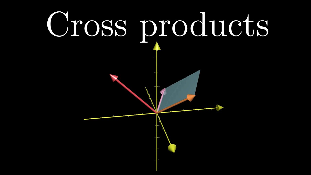
In the next chapter, you'll see another really good example of this duality in action as you and I get into the cross product.