How might LLMs store facts | Chapter 7, Deep Learning
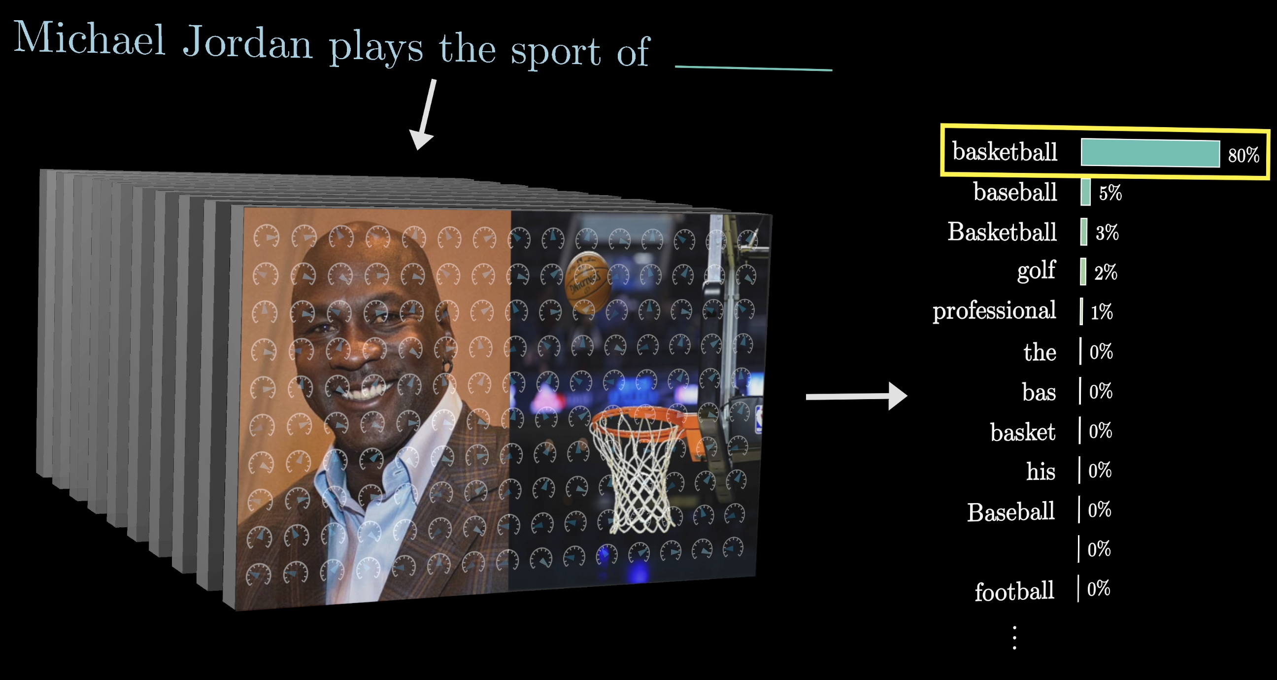
If you feed a large language model the phrase “Michael Jordan plays the sport of ___” and the model correctly predicts basketball as the following word, this would suggest that somewhere inside the model's hundreds of billions of parameters it has stored an association between a specific person and his specific sport.
In general, anyone who's played around with one of these models has a clear sense of the sheer amount of facts it has memorized.
Where are facts in LLMs stored?
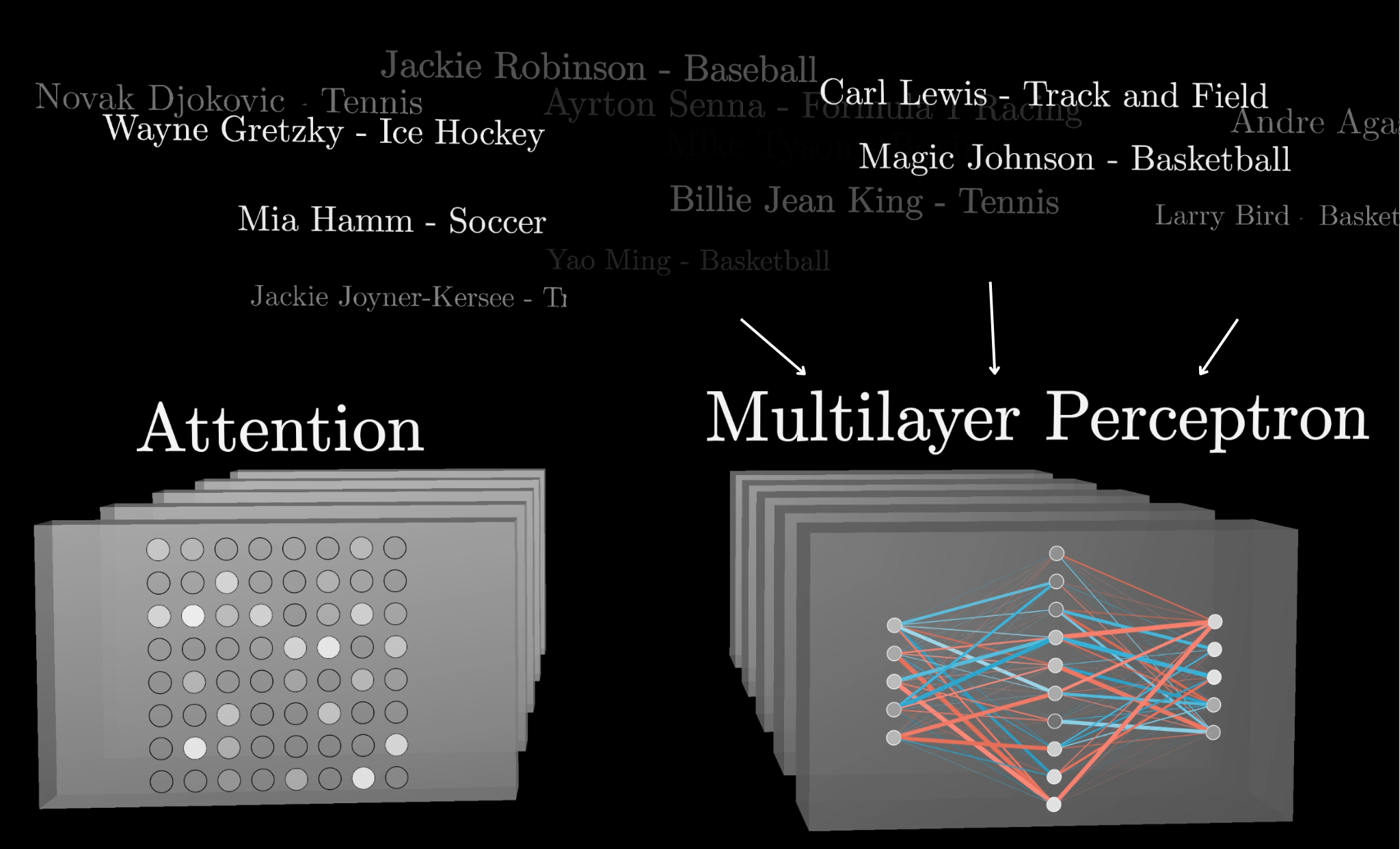
In December of 2023, a few researchers from Google DeepMind posted work on this question, using this same specific example of matching athletes to their sports. Although a full mechanistic understanding of how facts are stored remained unsolved, the researchers had reported some interesting partial results, including the very general high-level conclusion that facts seem to be stored inside a specific part of these networks known as the multi-layer perceptrons, often abbreviated as MLP.
In the last few chapters, you and I have been digging into the details of a transformer–the architecture underlying large language models.
In the previous chapter, we focused on a piece called attention. The next step for us is to unpack these multi-layer perceptrons, which make up the other big portion of the network.
Compared to attention, the computations in the MLPs are relatively simple, consisting essentially of a pair of matrix multiplications with a simple function in between. However, interpreting what these computations are doing is exceedingly challenging.

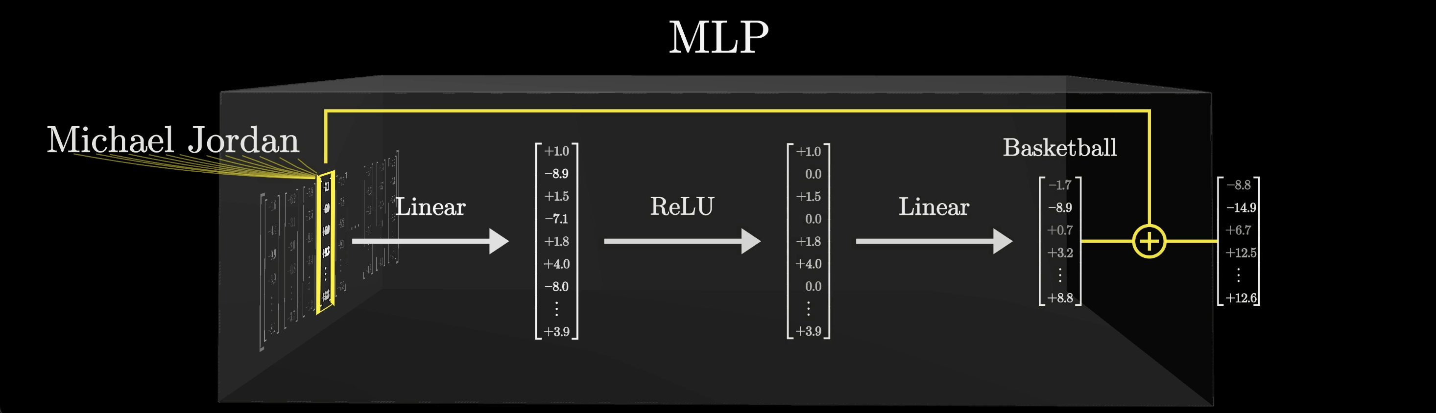
Our main goal in this lesson will be to step through the computations and make them memorable, but we'll do it in the context of showing a specific example of how one of these blocks could store a concrete fact. Specifically, it'll be storing the fact that Michael Jordan plays basketball.
In the last chapter, we've already covered how attention blocks let us incorporate context, but a majority of the model parameters live inside the MLP blocks. A common thought for what these MLP blocks might be doing is that they offer an extra capacity to store facts.
Assumptions
Before we dive into this example of how exactly the MLP could store the fact that Michael Jordan plays basketball, we're going to have to make a couple of assumptions about the high-dimensional space that we're working in.
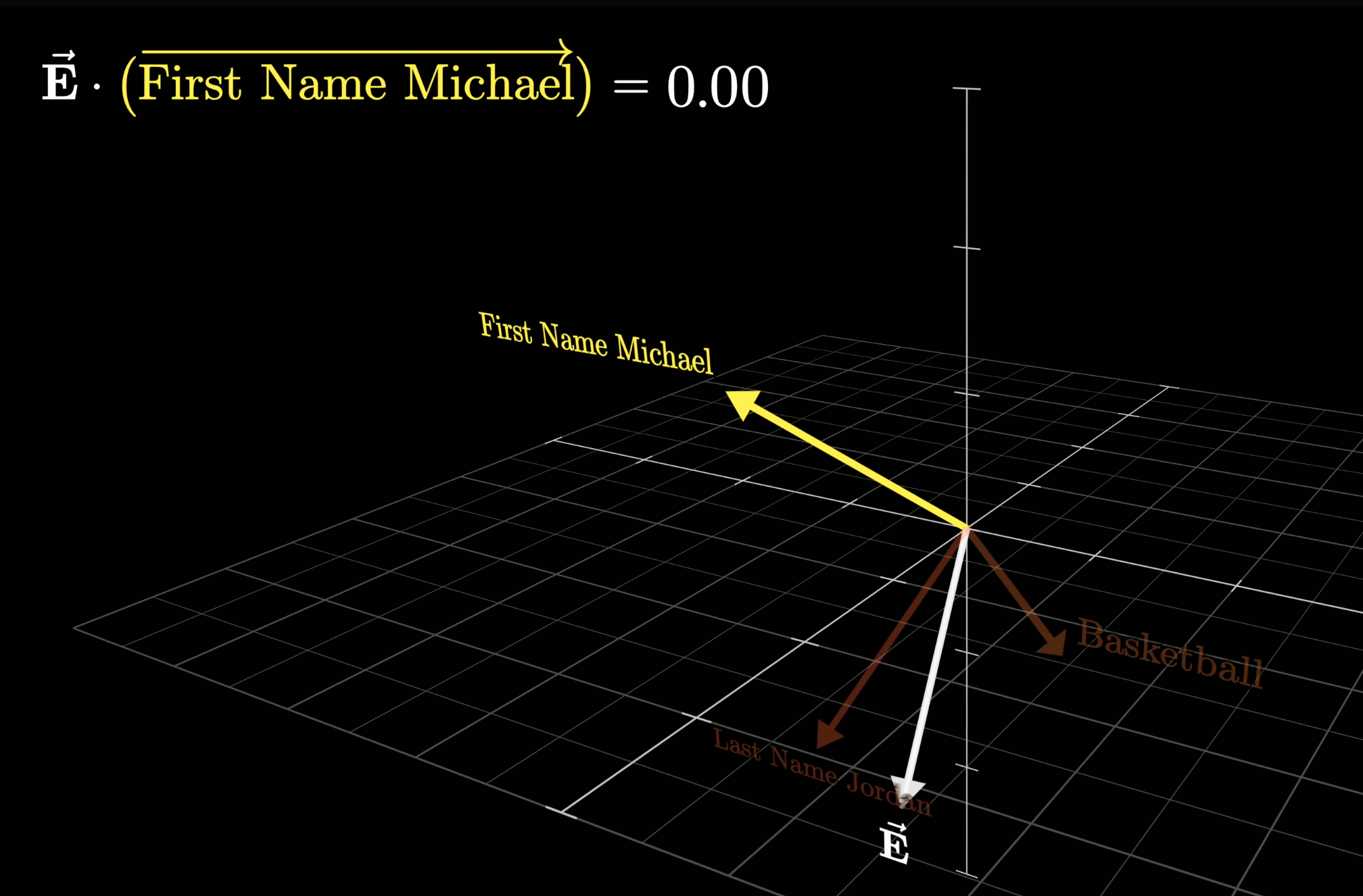
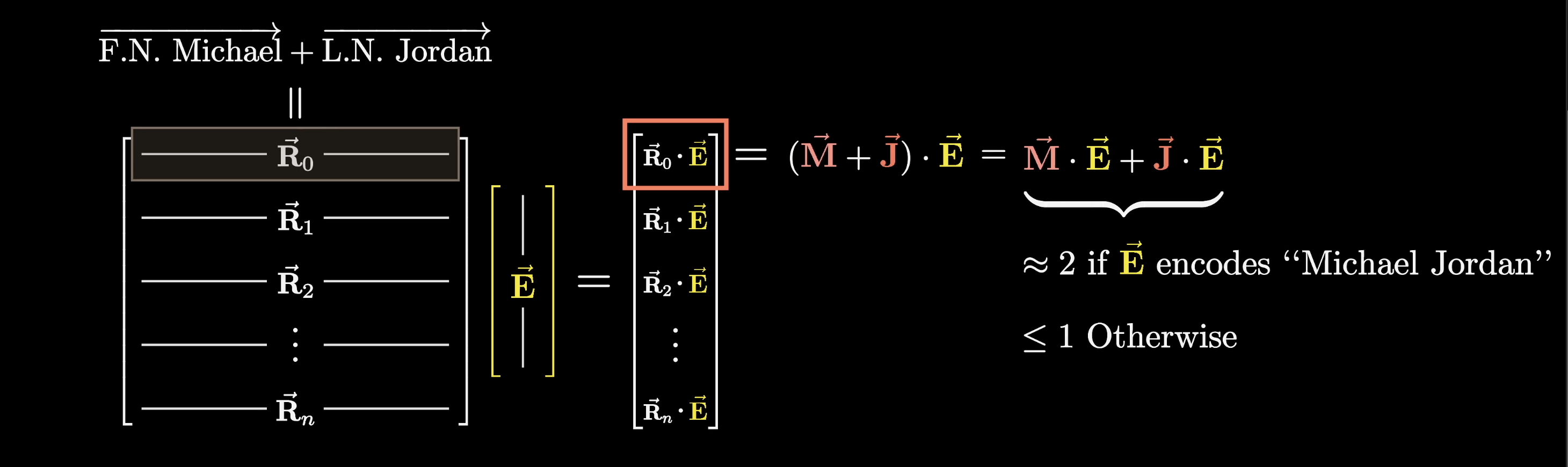
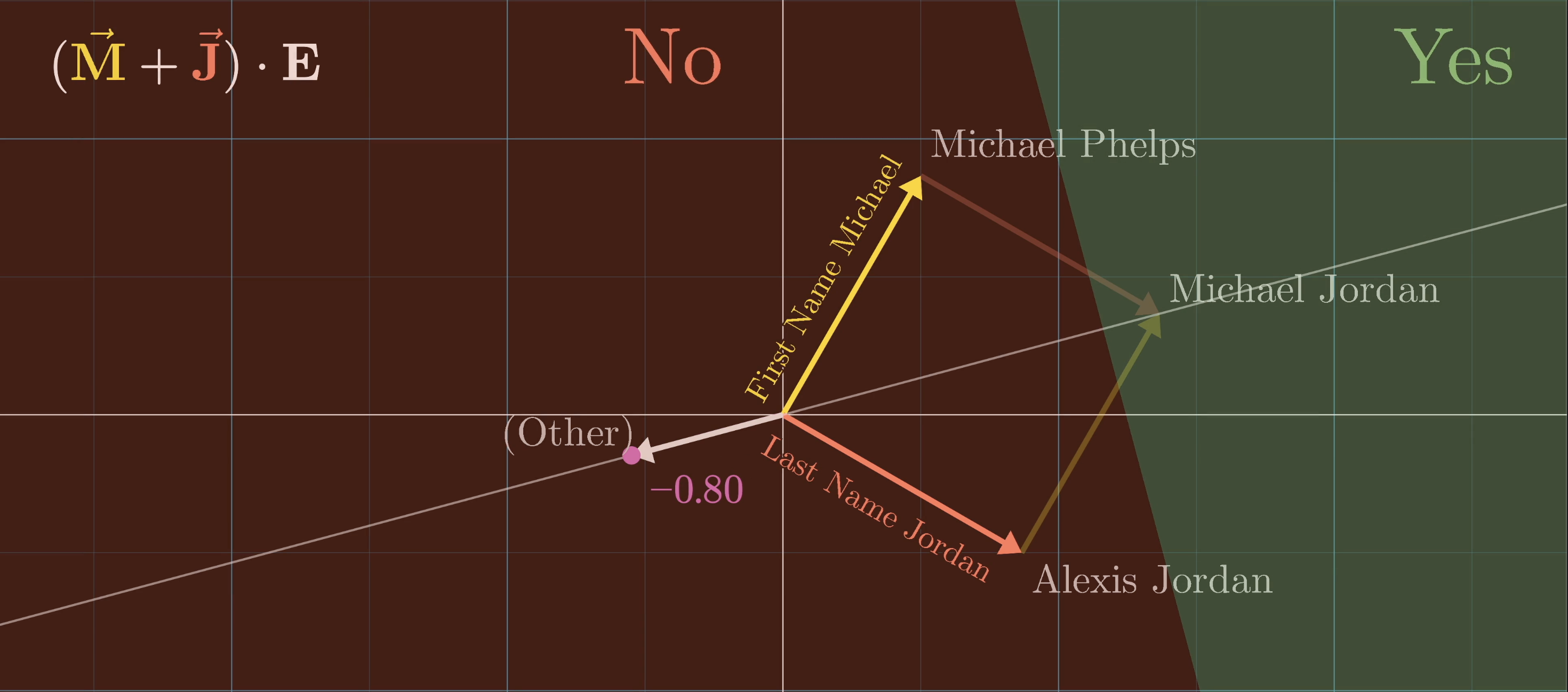
First, we'll suppose that one of the directions in this high-dimension space represents the idea of a first name Michael; another nearly perpendicular direction represents the idea of the last name Jordan; and a third, also nearly perpendicular, direction that represents the idea of basketball:
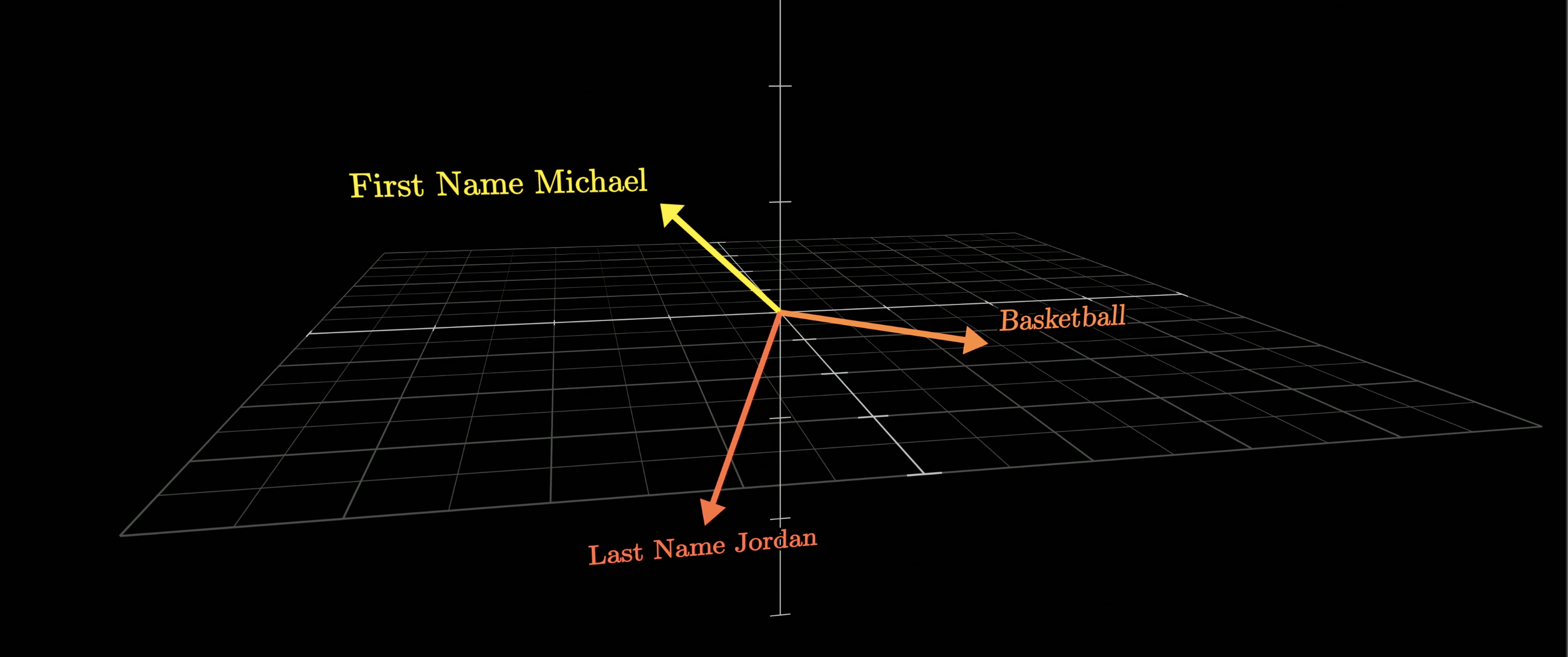
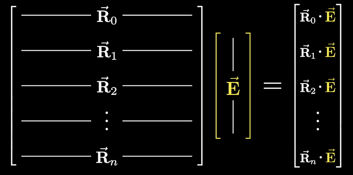
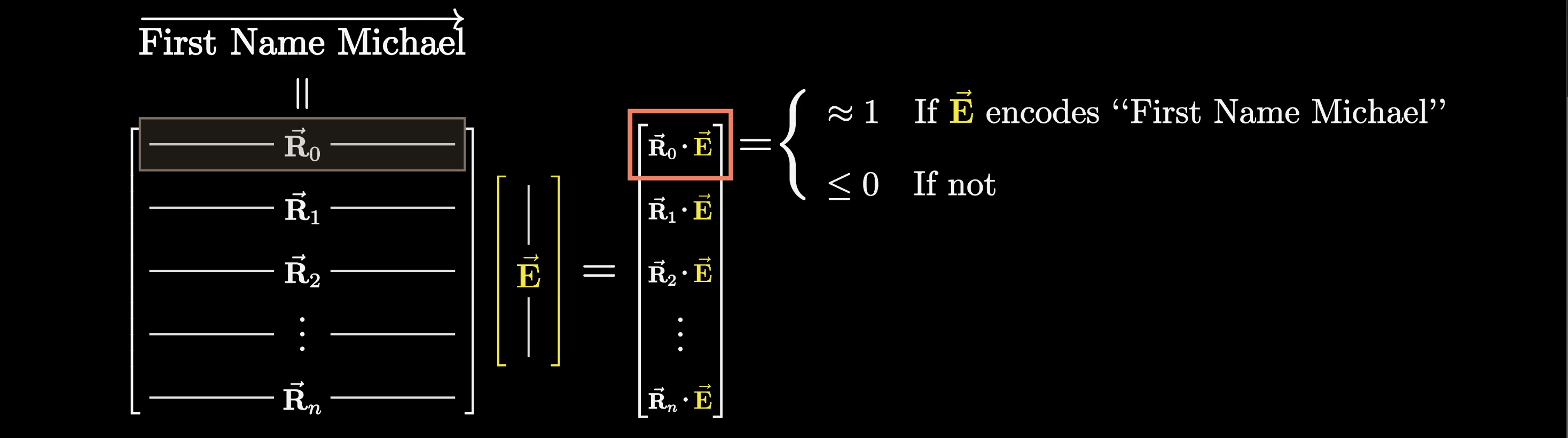
What this means is that, if we looked into the network and took out one of the vectors being processed, the dot product between one of the directions in this high-dimensional space and the vector will represent how well it aligns with the direction.
For example, if the dot product of the direction Michael and the vector is one, that would mean the vector encodes the idea of a person with the first name Michael. Otherwise, if the dot product were zero or negative, it would mean the vector doesn't really align with the Michael direction.
This vector aligns with the Micheal direction
This vector doesn't align with the Micheal direction
Similarly, its dot product with the other directions Jordan or basketball would tell you how well it aligns with those directions.
For simplicity, we'll completely ignore the very reasonable question of what it might mean if that dot product was bigger than one.
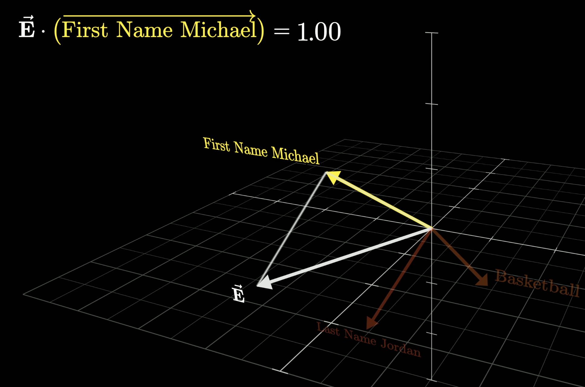
Now, let's think of a vector that is meant to represent the full name, Michael Jordan. Its dot product with both the directions Michael and Jordan would have to be one.
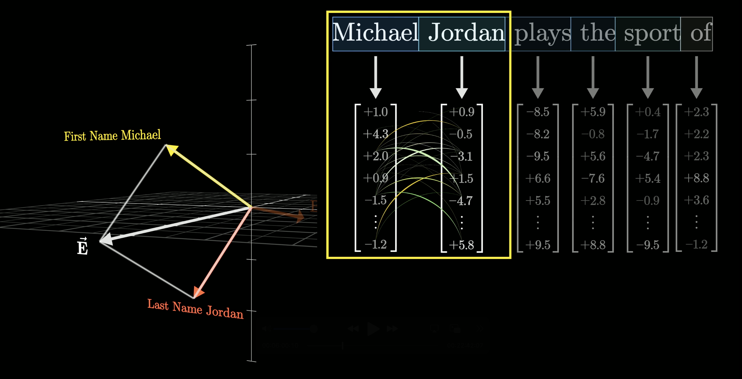
Since the text Michael Jordan spans two different tokens, Michael and Jordan, this would also mean we have to assume that an earlier attention block has successfully passed information to the second of these two vectors, Jordan, to ensure that it can encode both names.
With all that as the assumptions, let's now dive into the core of the lesson. What happens inside a multilayer perceptron?
Inside an MLP
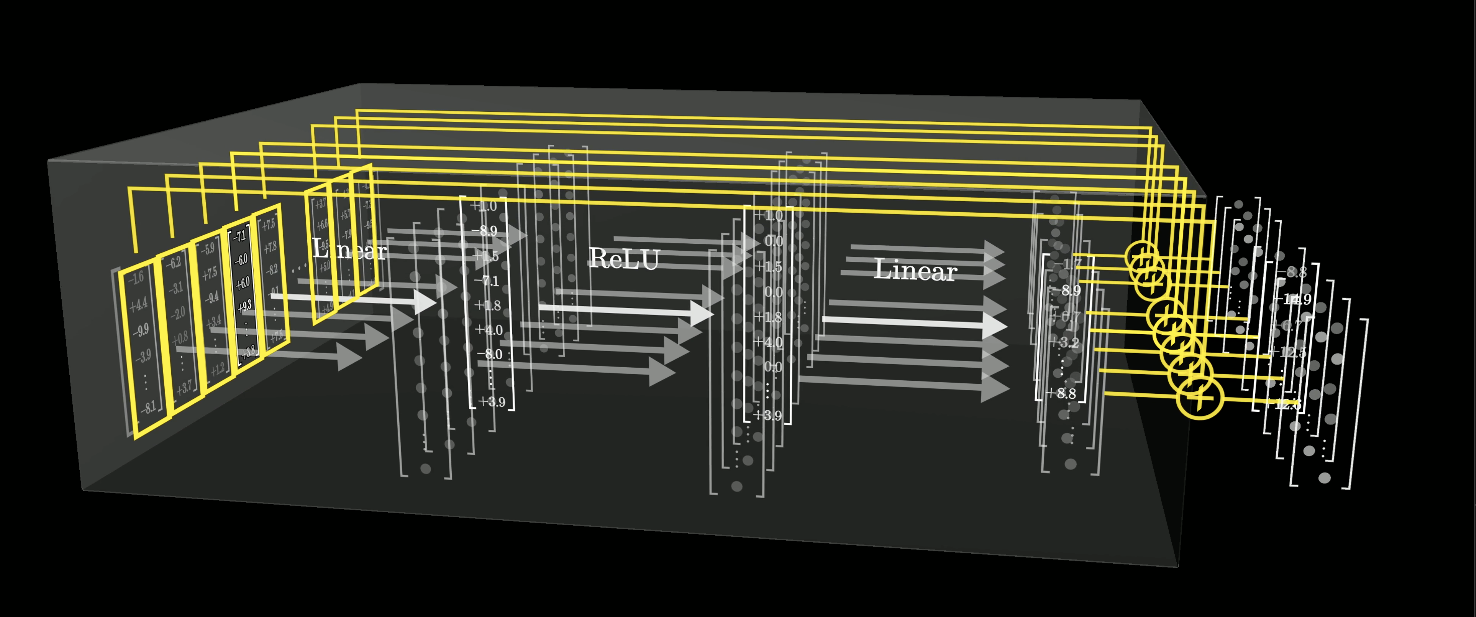
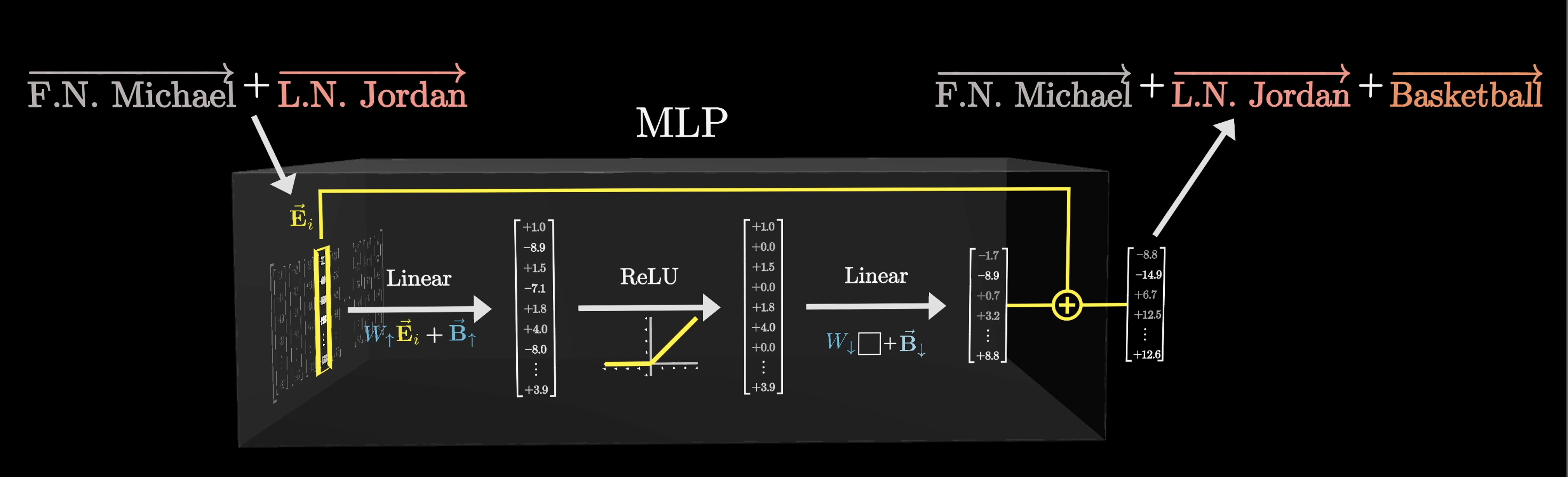
When entering the MLP block, each vector that was originally associated with one of the tokens from the input text is going to go through a short series of operations that will result in another vector of the same dimension.
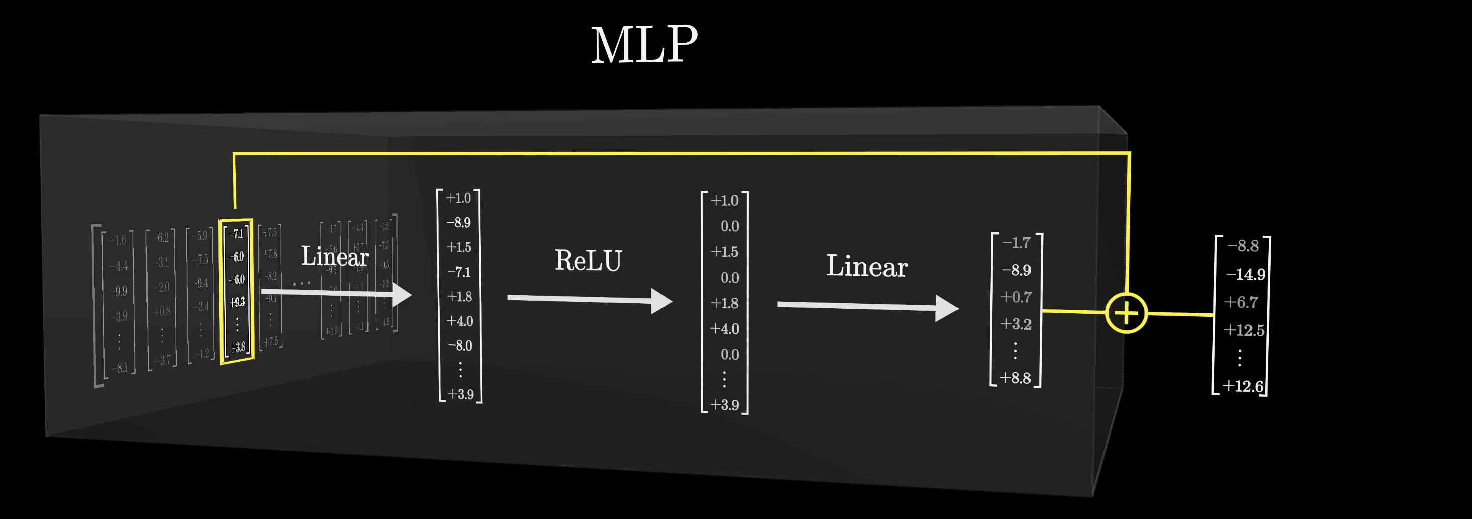
This sequence of operations is applied to every vector in the sequence and all happens in parallel.
We'll go over these operations in a moment, but after the operations, that resulting vector will be added to the original vector that flowed in, and that sum will be the result flowing out of the MLP.
What this means is that the vectors don't exchange information with each other in this step; they're all kind of doing their own thing. For us, this actually makes it a lot simpler to understand, as understanding what happens to just one of the vectors through this block will effectively help us understand what happens to all the vectors.
This sequence of operations is applied to every vector in the sequence and all happens in parallel.
Unlike the attention mechanism, the vectors passing through the MLP ____
When we say that this MLP block is going to encode the fact that Michael Jordan plays basketball, what we mean is that, if a vector that encodes the first name Michael and last name Jordan flows in the block, then we hope that the sequence of computations that exist in this block will produce an output, one that includes the direction basketball, to be added on to the vector encoding Michael Jordan.
Step 1
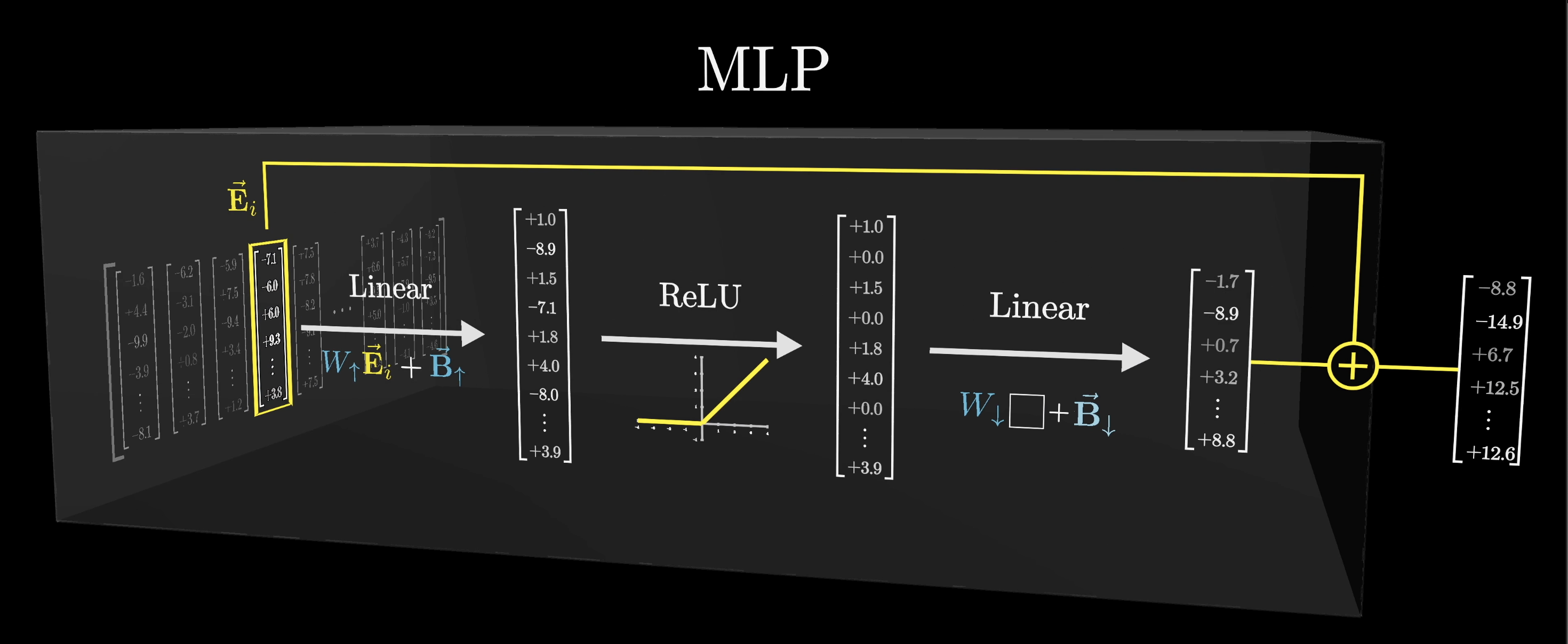
The first step of this MLP process looks like multiplying the vector that flowed into the MLP block by a very big matrix, which is no surprise when studying deep learning.
This matrix, like all of the other ones we've covered, is filled with model parameters that are learned from data. These parameters can be thought of as a bunch of knobs and dials that get tweaked and tuned to determine what the model behavior is.
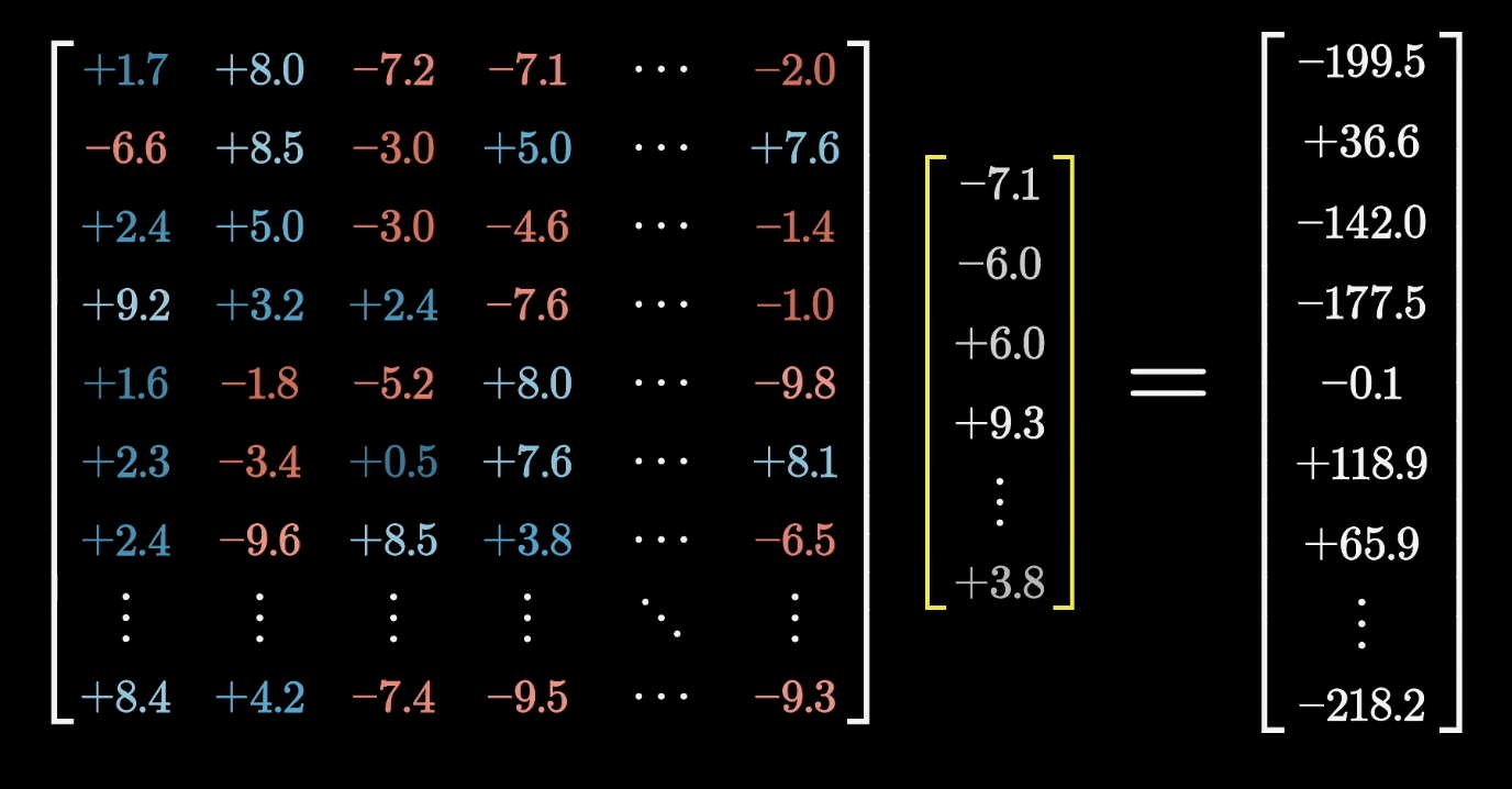
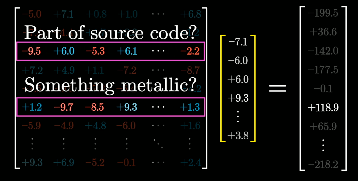
A nice way to think about matrix multiplication is to imagine each row of that matrix as being its own vector and taking a bunch of dot products between those rows and the vector being processed, which we'll label as .
For our example, let's suppose that the very first row happened to equal this first name Michael direction that we're presuming exists. That would mean that the first component in this output, the dot product , would equal one if that vector encodes the first name Michael, and zero or negative otherwise.
Even better, take a moment to think about what it would mean if that first row was this first name Michael plus last name Jordan direction, which for simplicity we'll write as .
As we take the dot product of with this embedding , things distribute really nicely, resulting in .
Notice how the value of this dot product would be two if the vector encodes the full name Michael Jordan, and otherwise it would be less than or equal to one.
This is just one row in this matrix. We might think of all of the other rows as asking some other kinds of questions in parallel, probing at some other sorts of features of the vector being processed.
Bias
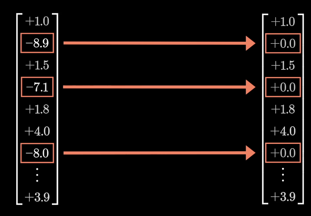
This first step of the MLP block also involves adding another vector to the output, known as the bias vector. This vector is also full of model parameters learned from data.
For our example, let's imagine that the value of this bias in that very first component is -1, meaning our final output looks like that relevant dot product, but minus one.
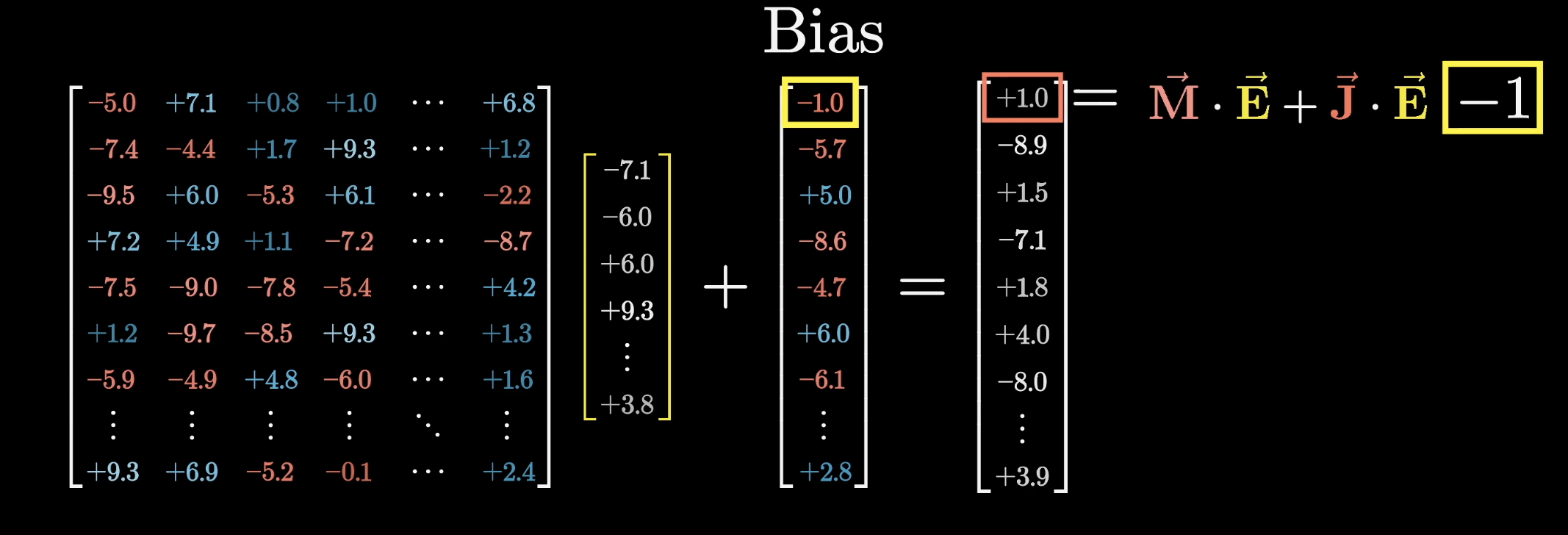
You might very reasonably wonder why we would want to assume that the model has learned this, and in a moment you'll see why it'll turn out very clean if we have a value here that is positive if and only if a vector encodes the full name Michael Jordan.
The total number of rows in this matrix is something like the number of questions being asked. In the case of GPT-3, whose numbers we've been following, is just under 50,000 and is exactly four times the number of dimensions in this embedding space. There's no specific reason why. You could make it more; you could make it less, but having a clean multiple tends to be friendly for hardware.
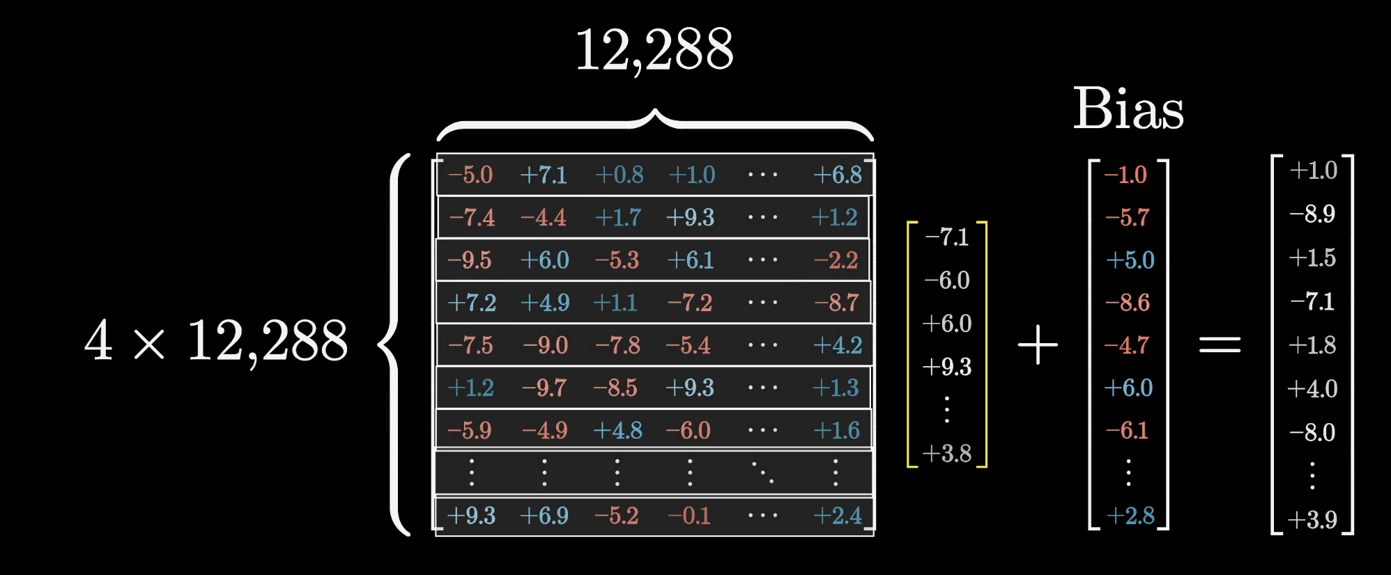
Since this matrix maps us into a higher dimensional space, we're going to label it as . We'll continue labeling the vector we're processing as , and we'll label this bias vector as .
At this point, a problem is that this operation is purely linear, but language is a very non-linear process. If the entry that we're measuring is high for Michael Jordan, it would also be somewhat triggered by Michael Phelps or Alexis Jordan, despite those being unrelated conceptually. What we really want is a simple yes/no for the full name Michael Jordan.
Rectified Linear Unit (ReLU)
In order to obtain this simple yes/no answer, the next step in this process is to pass this large intermediate vector through a very simple non-linear function. A common choice is one known as the Rectified Linear Unit, or ReLU for short. If you pass in a negative value, it returns a zero, and if you pass in a positive value, it leaves it unchanged.
Consider our imagined example where this first entry of the intermediate vector is one if and only if the full name is Michael Jordan and zero or negative otherwise, after you pass it through the ReLU, we can simply say that it is zero otherwise, as all the negative values get clipped to zero.
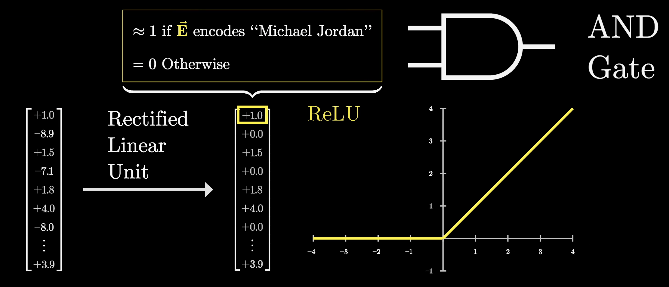
This function very directly mimics the behavior of an AND gate.
Often models will use a slightly modified function called GELU, which has the same basic shape but is just a bit smoother. For the purpose of this lesson, it's a little bit cleaner if we only think about the ReLU.
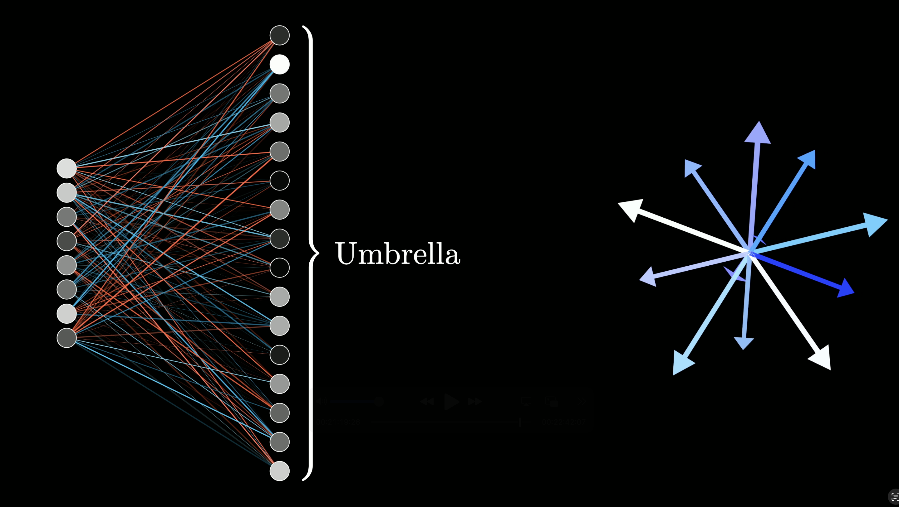
Neurons
When people refer to the neurons of a transformer, they're referring to the values leaving this ReLU.
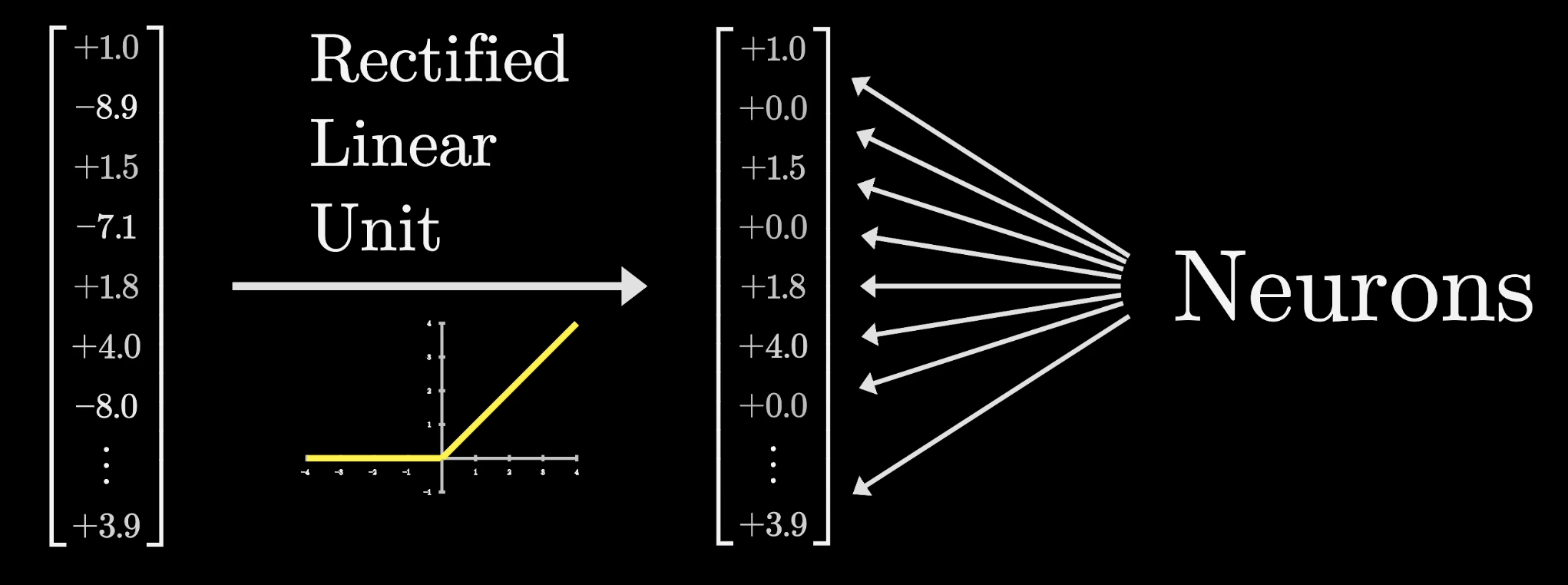
Whenever you see that common neural network picture with a layer of dots and a bunch of lines connecting to the previous layer, which we had in the earlier lessons of this series, it's typically meant to convey this combination of a linear step, a matrix multiplication, followed by some simple term-wise nonlinear function like a ReLU.
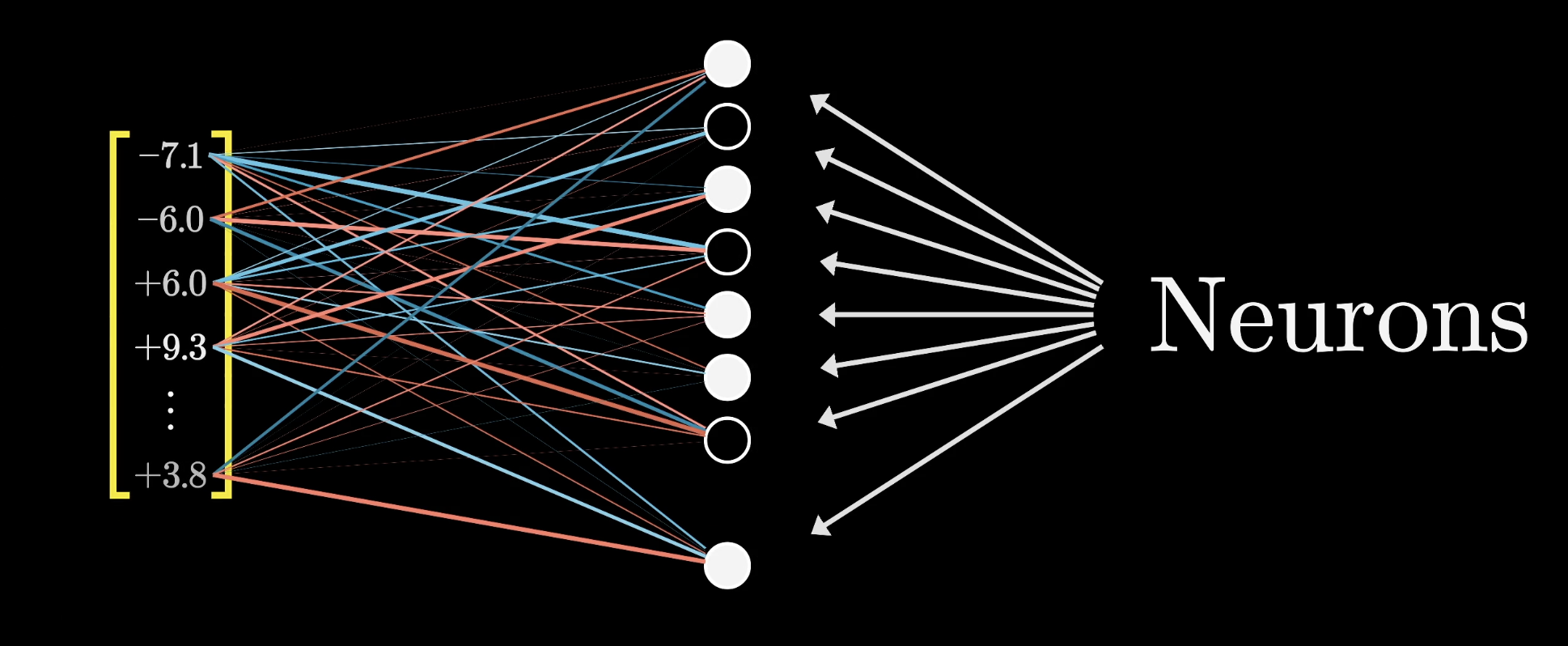
A neuron would be called active whenever this value is positive and inactive if that value is zero. In the image above, the white dots symbolize a neuron being active.
Using the GPT-3 numbers, how many parameters does the ReLU function require?
Third Step
The next step in this MLP process looks very similar to the first one. The vector leaving the ReLU would be multiplied by a very large matrix, followed by adding a certain bias vector. However, in this case, the number of dimensions in the output is back down to the size of the initial embedding space. We'll denote this matrix as the down projection matrix.
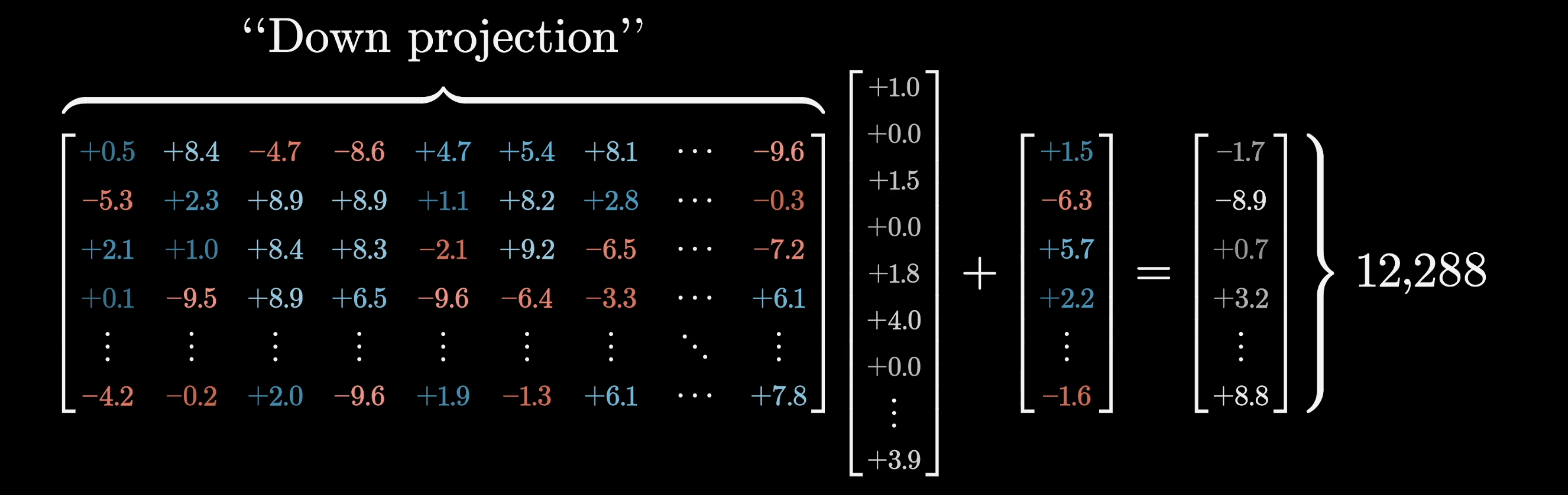
This time, instead of thinking of things row by row, it's nicer to think of it column by column.
Another way to conceptually think of matrix multiplication is by taking each column of the matrix and multiplying it by the corresponding term in the vector that it's processing, and then adding together all of those rescaled columns.
The reason it's nicer to think about it this way is because here the columns have the same dimension as the embedding space, so we can think of the columns as directions in that space. For instance, let's imagine that the model has learned to make that first column of this matrix into this basketball direction that we suppose exists.
What that would mean is that when the relevant neuron in that first position is active, we would be adding this Basketball column to the final result. But if that neuron was inactive, if that number was zero, then this would have no effect.
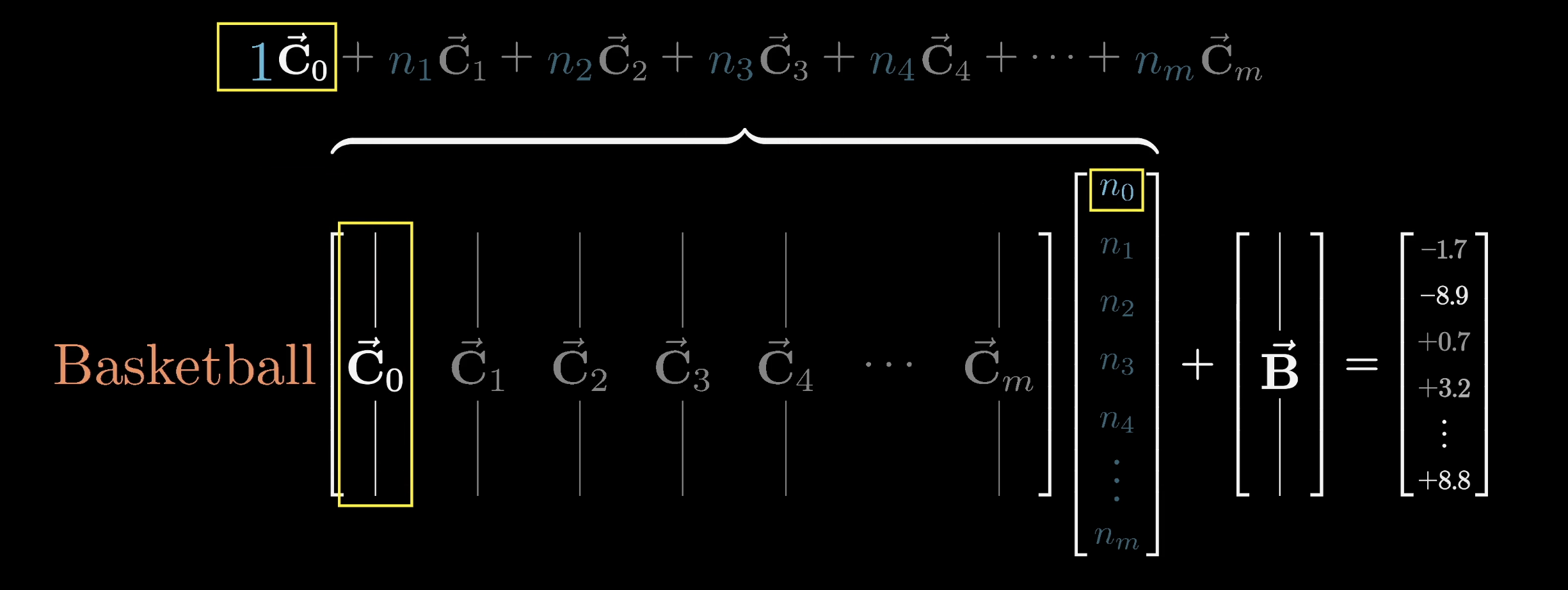
It doesn't just have to be basketball. The model could also bake into this column many other features that it wants to associate with something that has the full name Michael Jordan, like the Chicago Bulls, or the number 23. On top of that, all of the other columns in this matrix tell you what will be added to the final result if the corresponding neuron is active.
If you have a bias in this case, it's something that's added on regardless of the neuron values. For now, feel free to ignore it, as it's kind of hard to say exactly what it's doing, just like all other parameter-filled objects. We'll label this down projection matrix as and this bias vector as .
As we previewed earlier, the result of the last linear step is added to the one that flowed into the block at that position, and that returns the final result.
For example, if the vector flowing in encoded both first name Michael and last name Jordan, then because this sequence of operations will trigger what is effectively an AND gate, it will add on the basketball direction and result in a vector that encodes all of those together.
Remember, this is a process happening to every one of those vectors in parallel, not just this one vector. In particular, taking the GPT-3 numbers, the number of neuron activations in one of these blocks is not just 50,000, it’s 50,000 times the number of tokens in the input.
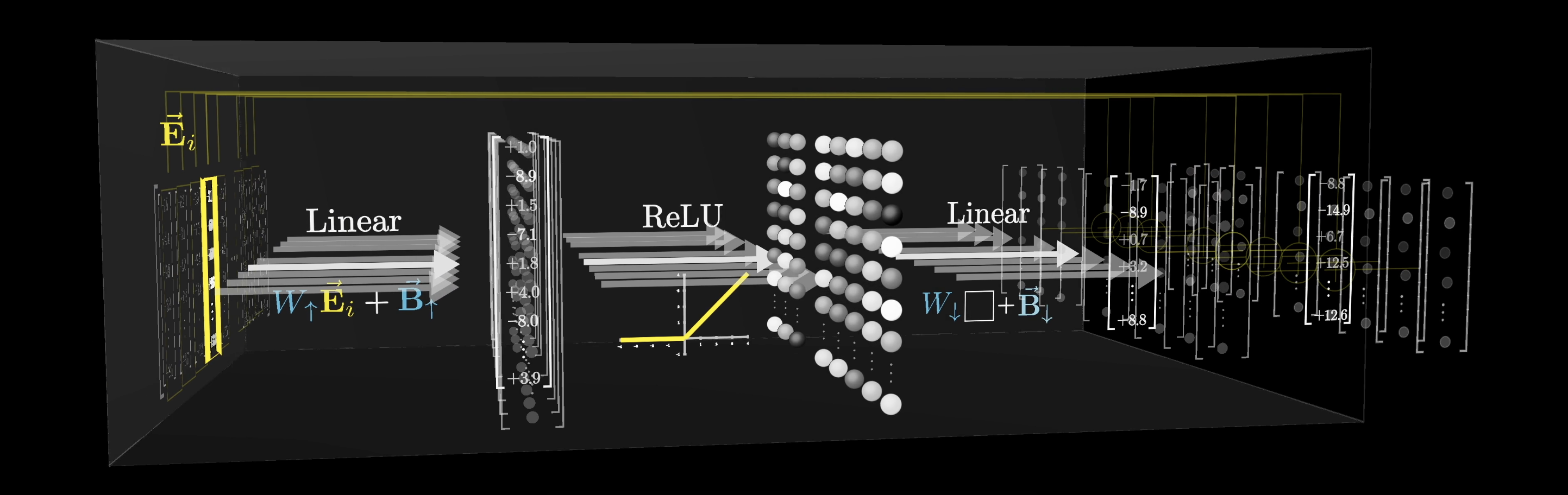
And that’s it! That’s all there is to an MLP: Two matrix products, each with a bias added, and a simple clipping function in between.
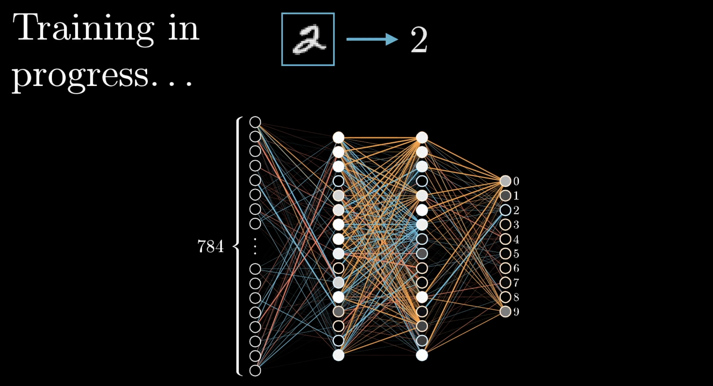
If any of you have watched the earlier videos of the series, you will recognize this structure as the most basic kind of neural network that we studied there. In the previous example, the neural network was trained to recognize handwritten digits.
In the context of a transformer for a large language model, this is one piece in a much larger architecture. Any attempt to interpret what exactly it's doing is heavily intertwined with the idea of encoding information into vectors of a high-dimensional embedding space.
But before we conclude the lesson, I do want to step back and reflect on two different things, the first of which is a kind of bookkeeping, and the second of which involves a very thought-provoking fact about higher dimensions.
Counting Parameters
In the last two chapters, we started counting up the total number of parameters in GPT-3 and seeing exactly where they live, so let's quickly finish it up here. We already mentioned how this up projection matrix, , has just under 50,000 rows and that each row matches the size of the embedding space, which for GPT-3 is 12,288. Multiplying those together gives us 604 million parameters just for that matrix. The down projection matrix, , has the same number of parameters, just with a transposed shape, giving us another 604 million parameters.
Together, these two matrices contain about 1.2 billion parameters. While the bias vector does also account for a couple more parameters, it's a trivial proportion of the total, so we’ll disregard it.

That's not all. In GPT-3, this sequence of embedding vectors flows through not one, but 96 distinct MLPs, so the total number of parameters devoted to all of these blocks adds up to about 116 billion. This is around two-thirds of the total parameters in the network, and when you add it to everything that we had before, for the attention blocks, the embedding, and the unembedding, you do indeed get that grand total of 175 billion parameters.
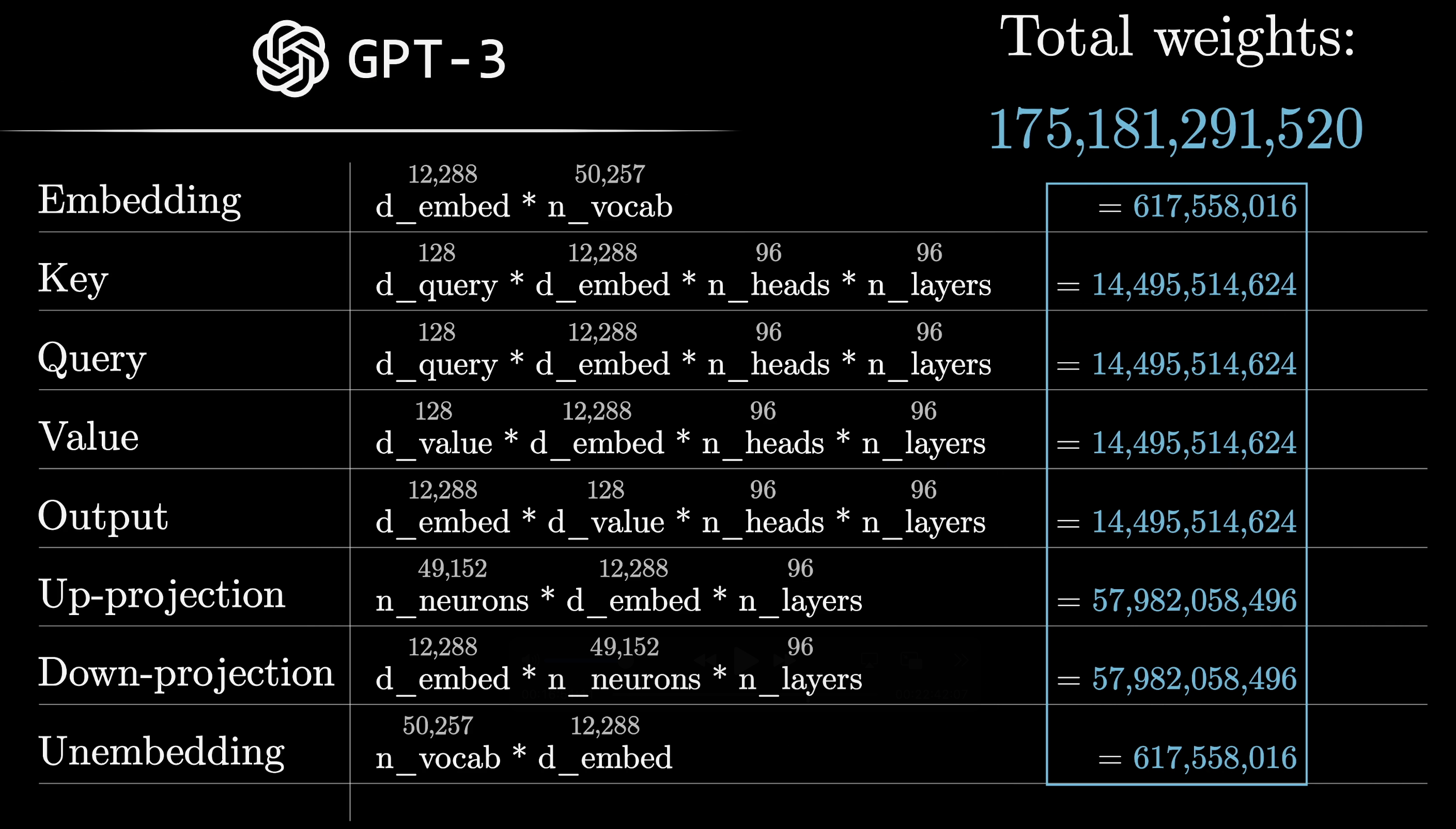
It's worth mentioning that there's another set of parameters associated with those normalization steps that this explanation has skipped over, roughly accounting for 49,000 parameters, but just like the bias vector, they account for a very trivial proportion of the total amount.
As to that second point of reflection, you might be wondering if this central Michael Jordan example we've been spending so much time on actually reflects how facts are stored in real large language models.
It is true that the rows of that first matrix can be thought of as directions in this embedding space, and that means the activation of each neuron tells you how much a given vector aligns with some specific direction. It is also true that the columns of that second matrix tell you what will be added to the result if that neuron is active.
However, evidence suggests that individual neurons very rarely represent a single clean feature like Michael Jordan, and there may actually be a very good reason that this is the case. It's related to an idea known to interpretability researchers as superposition, and it might help to explain both why the models are especially hard to interpret as well as why they scale surprisingly well.
Superposition
The basic idea is that if you have an n-dimensional space and you want to represent a bunch of different features using directions that are all perpendicular to one another in that space (that way if you add a component in one direction it won't influence any of the other directions) then the maximum number of vectors you can fit is only n, the number of dimensions.
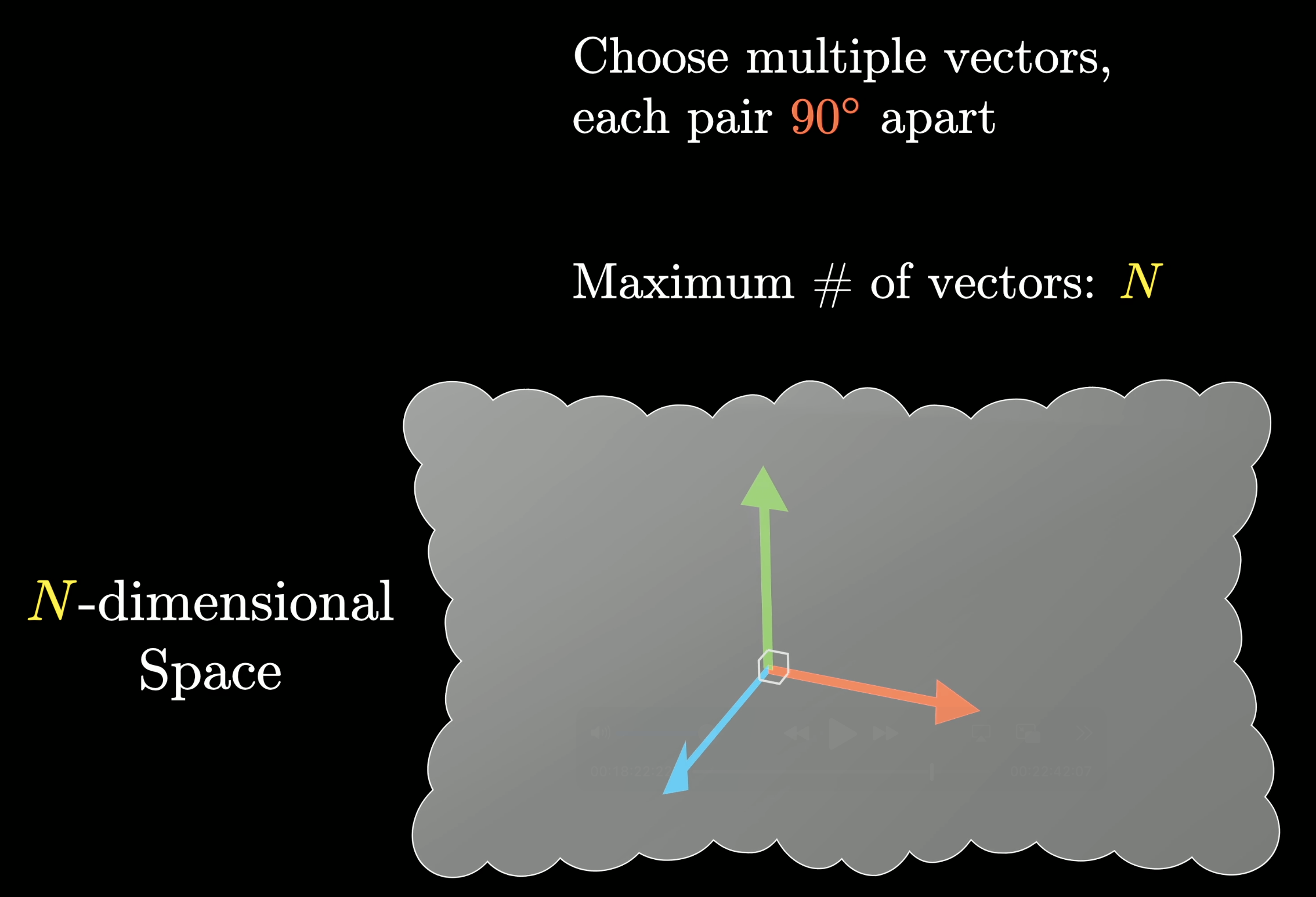
To a mathematician this is the definition of dimension!
However, what if you relax that constraint a little bit and tolerate some noise? Say you allow those features to be represented by vectors that aren't exactly perpendicular; they're just nearly perpendicular, maybe between 85 and 95 degrees apart.
For smaller dimensions, this hardly gives you any extra wiggle room to fit more vectors in, which makes it all the more counterintuitive that, for higher dimensions, the answer changes dramatically.
In general, a consequence of something known as the Johnson-Lindenstrauss lemma is that the number of vectors that can be crammed into a space that are nearly perpendicular grows exponentially with the number of dimensions.

A Quick Demo
For the video version of this lesson, I pulled up some quick and scrappy Python to demonstrate. However, in the video I made an error. I started by taking 10,000 distinct vectors, each of 100 dimensions. They begin at random, and here is a blot of what all the angles between pairs of those vectors look like.
Even though these are randomly chosen, you can already see how with a higher dimension, there is a bias towards pairs being closer to 90 degrees apart.
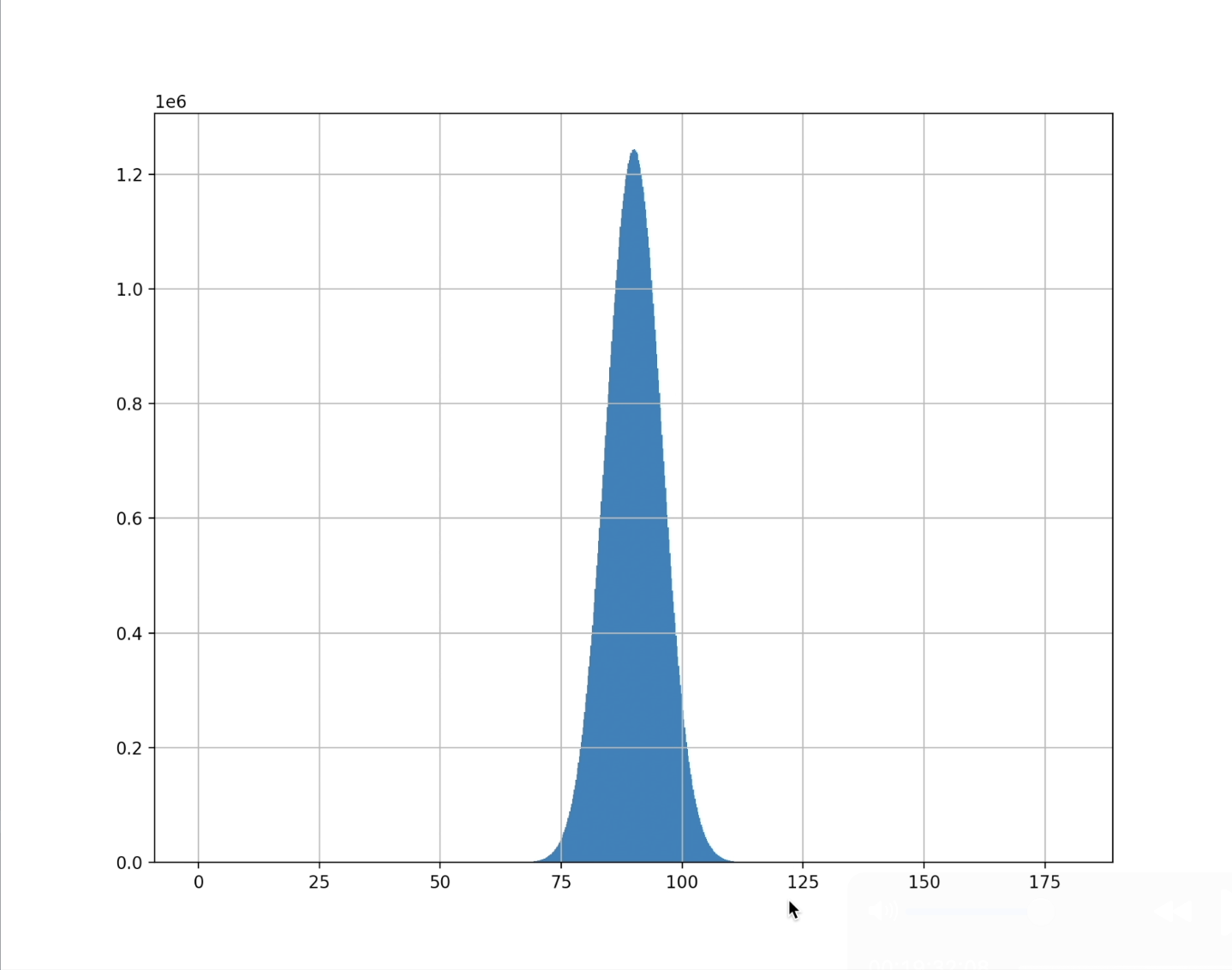
I then ran a certain optimization process to iteratively nudge these vectors to try to become more perpendicular to each other, and in the end, this was the distribution.
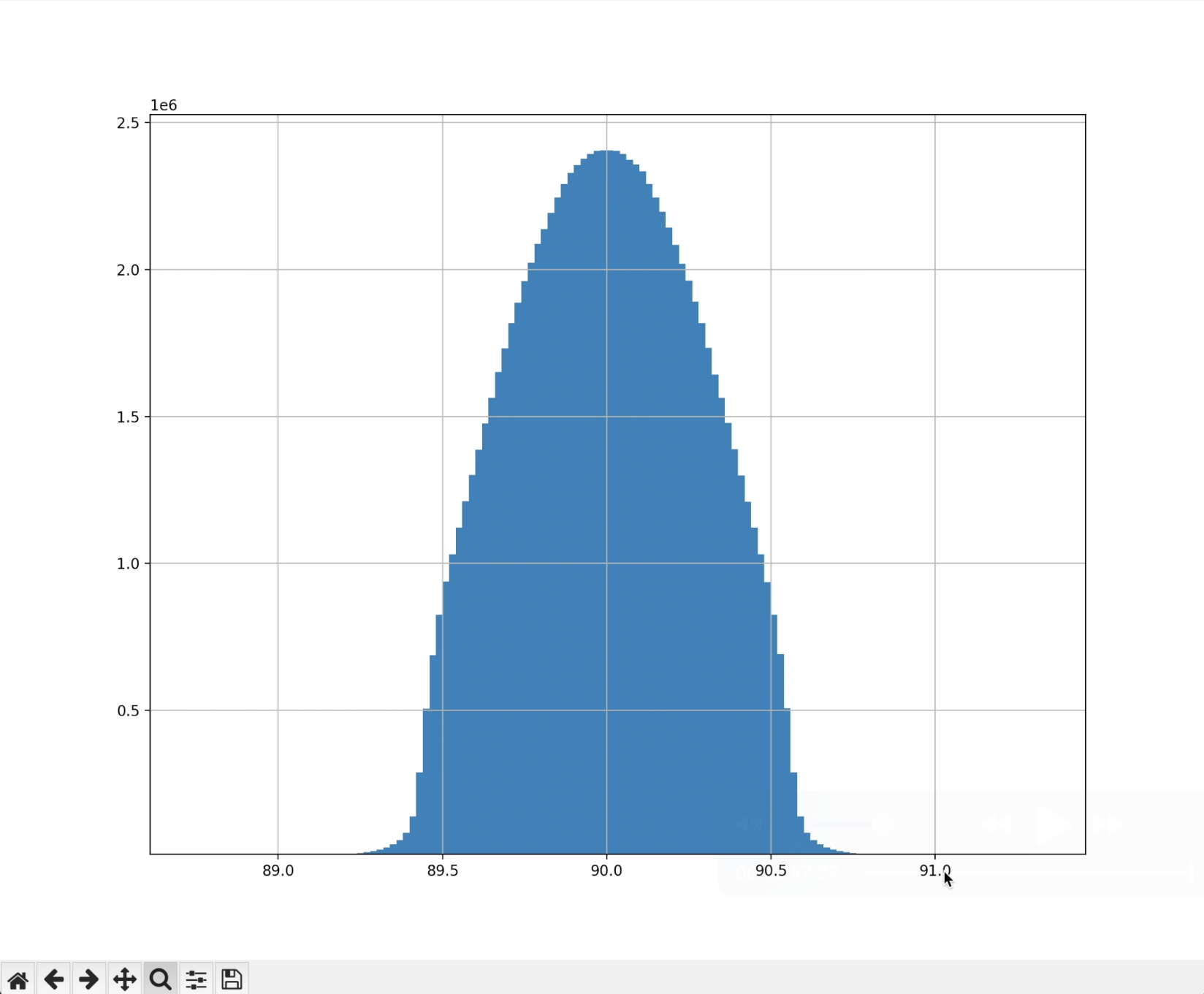
All the angles are between 89 and 91. Amazing! That’s 10,000 vectors, all being crammed to be nearly perpendicular in a space with 100 times fewer dimensions.
However, there was a mistake in the code and it looks like what was really happening is that a few pairs get shot out to have dot products near ±1, hiding in the wings of the plot. I was using a bad cost function that didn't appreciably punish those cases. On closer inspection, I think it's not actually possible to get 100,000 vectors in 100 dimensions to be as "nearly orthogonal" as this. 100 dimensions are not enough, at least for the (89°, 91°) range, for the Johnson-Lindenstrauss lemma to really kick in.
The broader point made at that point in the video is true, though, which is that the number of nearly orthogonal vectors you can cram in will scale exponentially. But when that makes for an appreciable effect is an interesting question. The viewer Nick Yoder wrote in with more explorations on this, with these as a few highlights:
- Forcing pairs of vectors into the range (89°, 91°) is rather tight. At this angle, things don't get interesting until dimensions > 250,000
- 85 degrees (dot product of only 0.087) scales VERY quickly
- 85 degrees and 12,288 dimensions (GPT3 embedding space) holds well over 40 Billion vectors (likely more than )
- 85 degrees and 116,000 dimensions (within reason for GPT4, GPT-o1, -o3 or similar newer models) holds well over a Googol () vectors and likely over
This point is very significant for large language models, which benefit from associating independent ideas with nearly perpendicular directions. It means that it's possible for the models to store many, many more ideas than there are dimensions in the space that it's allotted. This might explain why model performance seems to scale so well with size.
A space that has 10 times as many dimensions can store way, way more than 10 times as many independent ideas.
And this is relevant not just to the embedding space of the model, but also to that vector full of neurons in the middle of that multilayer perceptron that we just studied. In our case, at the sizes of GPT-3, it might not just be probing at 50,000 features. If it instead leveraged this enormous added capacity by using nearly perpendicular directions of the space, it could be probing at orders of magnitude more features of the vector being processed.
In doing so, it means that individual features aren't going to be visible as a single neuron lighting up. It would have to look like some specific combination of neurons instead, hence a superposition.
How does the concept of superposition help large language models like GPT-3 store and process more features than the number of dimensions in their vector space?
Additional Resources
For any of you curious to learn more, a key relevant search term here is sparse autoencoder, which is a tool that some of the interpretability people use to try to extract what the true features are, even if they're very superimposed on all these neurons.
Here are the links to some really great anthropic posts all about this.
At this point, we haven't touched every detail of a transformer, but we have hit the most important points. The main thing that we will want to cover in the next chapter is the training process. The short answer for how the training process works is that it's all backpropagation, and we covered backpropagation in a separate context with earlier chapters in the series. But there is more to discuss, like the specific cost function used for language models, the idea of fine-tuning using reinforcement learning with human feedback, and the notion of scaling laws.
Thanks
Special thanks to those below for supporting the original video behind this post, and to current patrons for funding ongoing projects. If you find these lessons valuable, consider joining.